

Stationary Kernels

Stationary kernels can be expressed as a function of the difference between their inputs.

$C(\mathbf{x}, \mathbf{y}) = K(||\mathbf{x} - \mathbf{y}||_{p})$

Note that any norm may be used to quantify the distance between the two vectors $\mathbf{x} \ \& \ \mathbf{y}$ . The values $p = 1$ and $p = 2$ represent the Manhattan distance and Euclidean distance respectively.

Instantiating Stationary Kernels

Stationary kernels are implemented as a subset of the StationaryKernel[T, V, M] class which requires a Field[T] implicit object (an algebraic field which has definitions for addition, subtraction, multiplication and division of its elements much like the number system). You may also import spire.implicits._ in order to load the default field implementations for basic data types like Int, Double and so on. Before instantiating any child class of StationaryKernel one needs to enter the following code.

    import spire.algebra.Field
    import io.github.mandar2812.dynaml.analysis.VectorField
    //Calculate the number of input features
    //and create a vector field of that dimension
    val num_features: Int = ...
    implicit val f = VectorField(num_features)

Radial Basis Function Kernel¶

kernel

$C(\mathbf{x},\mathbf{y}) = exp\left(-\frac{||\mathbf{x}-\mathbf{y}||^2}{2\sigma^2}\right)$

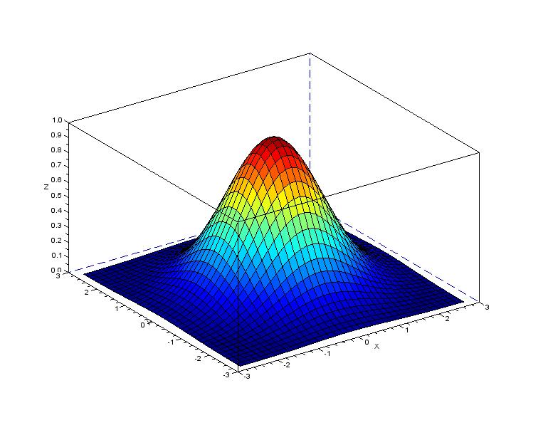
The RBF kernel is the most popular kernel function applied in machine learning, it represents an inner product space which is spanned by the Hermite polynomials and as such is suitable to model smooth functions. The RBF kernel is also called a universal kernel for the reason that any smooth function can be represented with a high degree of accuracy assuming we can find a suitable value of the bandwidth.

val rbf = new RBFKernel(4.0)

Squared Exponential Kernel¶

A generalization of the RBF Kernel is the Squared Exponential Kernel

$C(\mathbf{x},\mathbf{y}) = h \ exp\left(-\frac{||\mathbf{x}-\mathbf{y}||^2}{2l^2}\right)$

val rbf = new SEKernel(4.0, 2.0)

Mahalanobis Kernel¶

This kernel is a further generalization of the SE kernel. It uses the Mahalanobis distance instead of the Euclidean distance between the inputs.

$C(\mathbf{x},\mathbf{y}) = h \ exp\left(-\frac{1}{2}(\mathbf{x}-\mathbf{y})^\intercal \Sigma^{-1} (\mathbf{x}-\mathbf{y})\right)$

The Mahalanobis distance $(\mathbf{x}-\mathbf{y})^\intercal \Sigma^{-1} (\mathbf{x}-\mathbf{y})$ is characterized by a symmetric positive definite matrix $\Sigma$ . This distance metric reduces to the Euclidean distance if $\Sigma$ is the identity matrix. Further, if $\Sigma$ is diagonal, the Mahalanobis kernel becomes the Automatic Relevance Determination version of the SE kernel (SE-ARD).

In DynaML the class MahalanobisKernel implements the SE-ARD kernel with diagonal $\Sigma$ .

val bandwidths: DenseVector[Double] = _
val amp = 1.5

val maha_kernel = new MahalanobisKernel(bandwidths, amp)

Student T Kernel¶

$C(\mathbf{x},\mathbf{y}) = \frac{1}{1 + ||\mathbf{x}-\mathbf{y}||^d}$

val tstud = new TStudentKernel(2.0)

Rational Quadratic Kernel¶

$C(\mathbf{x},\mathbf{y}) = \left( 1 + \frac{||\mathbf{x}-\mathbf{y}||^2}{2 \mu \ell^2} \right)^{-\frac{1}{2} (dim(\mathbf{x})+\mu)}$

val rat = new RationalQuadraticKernel(shape = 1.5, l = 1.5)

Cauchy Kernel¶

$C(\mathbf{x},\mathbf{y}) = \frac{1}{1 + \frac{||\mathbf{x}-\mathbf{y}||^2}{\sigma^2}}$

val cau = new CauchyKernel(2.5)

Gaussian Spectral Kernel¶

$C(\mathbf{x},\mathbf{y}) = cos(2\pi \mu ||\mathbf{x}-\mathbf{y}||) \ exp(-2\pi^{2} \sigma^{2} ||\mathbf{x}-\mathbf{y}||^{2} )$

//Define how the hyper-parameter Map gets transformed to the kernel parameters
val encoder = Encoder(
  (conf: Map[String, Double]) => (conf("c"), conf("s")),
  (cs: (Double, Double)) => Map("c" -> cs._1, "s" -> cs._2))

val gsmKernel = GaussianSpectralKernel[Double](3.5, 2.0, encoder)

Matern Half Integer¶

The Matern kernel is an important family of covariance functions. Matern covariances are parameterized via two quantities i.e. order $\nu$ and $\rho$ the characteristic length scale. The general matern covariance is defined in terms of modified Bessel functions.

$C_{\nu}(\mathbf{x},\mathbf{y}) = \frac{2^{1-\nu}}{\Gamma(\nu)} \left(\sqrt{2\nu}\frac{d}{\rho}\right)^{\nu} K_{\nu}\left(\sqrt{2\nu}\frac{d}{\rho}\right)$

Where $d = ||\mathbf{x} - \mathbf{y}||$ is the Euclidean ( $L_2$ ) distance between points.

For the case $\nu = p + \frac{1}{2}, p \in \mathbb{N}$ the expression becomes.

$C_{\nu}(\mathbf{x},\mathbf{y}) = exp\left(-\sqrt{2\nu}\frac{d}{\rho}\right) \frac{\Gamma(p+1)}{\Gamma(2p+1)} \sum_{i = 0}^{p}{\frac{(p+1)!}{i!(p-i)!}\left(\sqrt{8\nu}\frac{d}{\rho}\right)^{p-i}}$

Currently there is only support for matern half integer kernels.

implicit ev = VectorField(2)
val matKern = new GenericMaternKernel(1.5, p = 1)

Wavelet Kernel¶

The Wavelet kernel (Zhang et al, 2004) comes from Wavelet theory and is given as

$C(\mathbf{x},\mathbf{y}) = \prod_{i = 1}^{d} h\left(\frac{x_i-y_i}{a}\right)$

Where the function h is known as the mother wavelet function, Zhang et. al suggest the following expression for the mother wavelet function.

$h(x) = cos(1.75x)exp(-\frac{1}{2}x^2)$

val wv = new WaveletKernel(x => math.cos(1.75*x)*math.exp(-1.0*x*x/2.0))(1.5)

Periodic Kernel¶

The periodic kernel has Fourier series as its orthogonal eigenfunctions. It is used when constructing predictive models over quantities which are known to have some periodic behavior.

$C(\mathbf{x},\mathbf{y}) = exp\left(-2 \ sin^{2}\left(\frac{\pi \omega ||\mathbf{x}-\mathbf{y}||}{l^2}\right)\right)$

val periodic_kernel = new PeriodicKernel(lengthscale = 1.5, freq = 2.5)

Wave Kernel¶

$C(\mathbf{x},\mathbf{y}) = \frac{\theta}{||\mathbf{x} - \mathbf{y}||^2} \times sin(\frac{||\mathbf{x} - \mathbf{y}||^2}{\theta})$

val wv_kernel = WaveKernel(th = 1.0)

Laplacian Kernel¶

The Laplacian kernel is the covariance function of the well known Ornstein Ulhenbeck process, samples drawn from this process are continuous and only once differentiable.

$\begin{equation} C(\mathbf{x},\mathbf{y}) = exp \left(-\frac{||\mathbf{x}-\mathbf{y}||_{1}}{2\beta}\right) \end{equation}$

val lap = new LaplacianKernel(4.0)