

Gaussian Processes

Gaussian Processes are stochastic processes whose finite dimensional distributions are multivariate gaussians.

Gaussian Processes are powerful non-parametric predictive models, which represent probability measures over spaces of functions. Ramussen and Williams is the definitive guide on understanding their applications in machine learning and a gateway to their deeper theoretical foundations.

Gaussian Process models are well supported in DynaML, the AbstractGPRegressionModel[T, I] and AbstractGPClassification[T, I] classes which extend the StochasticProcessModel[T, I, Y, W] base trait are the starting point for all GP implementations.

Gaussian Process Regression

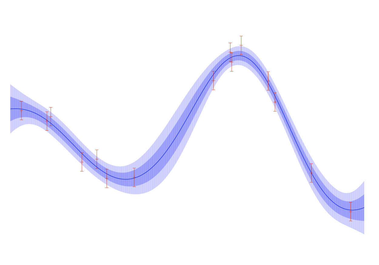
The GP regression framework aims to infer an unknown function $f(x)$ given $y_i$ which are noise corrupted observations of this unknown function. This is done by adopting an explicit probabilistic formulation to the multi-variate distribution of the noise corrupted observations $y_i$ conditioned on the input features (or design matrix) $X$

$$\begin{align} & y = f(x) + \epsilon \\ & f \sim \mathcal{GP}(m(x), C(x,x')) \\ & \left(\mathbf{y} \ \ \mathbf{f_*} \right)^T | X \sim \mathcal{N}\left(\mathbf{0}, \left[ \begin{matrix} K(X, X) + \sigma^{2} \it{I} & K(X, X_*) \\ K(X_*, X) & K(X_*, X_*) \end{matrix} \right ] \right) \end{align}$$

In the presence of training data

$$X = (x_1, x_2, \cdot , x_n) \ \mathbf{y} = (y_1, y_2, \cdot , y_n)$$

Inference is carried out by calculating the posterior predictive distribution over the unknown targets $\mathbf{f_*}|X,\mathbf{y},X_*$ assuming $X_*$, the test inputs are known.

$$\begin{align} & \mathbf{f_*}|X,\mathbf{y},X_* \sim \mathcal{N}(\mathbf{\bar{f_*}}, cov(\mathbf{f_*})) \label{eq:posterior}\\ & \mathbf{\bar{f_*}} \overset{\triangle}{=} \mathbb{E}[\mathbf{f_*}|X,y,X_*] = K(X_*,X)[K(X,X) + \sigma^{2}_n \it{I}]^{-1} \mathbf{y} \label{eq:posterior:mean} \\ & cov(\mathbf{f_*}) = K(X_*,X_*) - K(X_*,X)[K(X,X) + \sigma^{2}_n \it{I}]^{-1}K(X,X_*) \end{align}$$

GP models for a single output

For univariate GP models (single output), use the GPRegression class (an extension of AbstractGPRegressionModel). To construct a GP regression model you would need:

• Training data
• Kernel/covariance instance to model correlation between values of the latent function at each pair of input features.
• Kernel instance to model the correlation of the additive noise, generally the DiracKernel (white noise) is used.

val trainingdata: Stream[(DenseVector[Double], Double)] = ...
val num_features = trainingdata.head._1.length

// Create an implicit vector field for the creation of the stationary
// radial basis function kernel
implicit val field = VectorField(num_features)

val kernel = new RBFKernel(2.5)
val noiseKernel = new DiracKernel(1.5)
val model = new GPRegression(kernel, noiseKernel, trainingData)

GP models for multiple outputs

As reviewed in Lawrence et.al, Gaussian Processes for multiple outputs can be interpreted as single output GP models with an expanded index set. Recall that GPs are stochastic processes and thus are defined on some index set, for example in the equations above it is noted that $x \in \mathbb{R}^p$ making $\mathbb{R}^p$ the index set of the process.

In case of multiple outputs the index set is expressed as a cartesian product $x \in \mathbb{R}^{p} \times \{1,2, \cdots, d \}$, where $d$ is the number of outputs to be modeled.

It needs to be noted that now we will also have to define the kernel function on the same index set i.e. $\mathbb{R}^{p} \times \{1,2, \cdots, d \}$.

In multi-output GP literature a common way to construct kernels on such index sets is to multiply base kernels on each of the parts $\mathbb{R}^p$ and $\{1,2,\cdots,d\}$, such kernels are known as separable kernels.

$$\begin{equation} K((\mathbf{x}, d), (\mathbf{x}', d')) = K_{x}(\mathbf{x}, \mathbf{x}') . K_{d}(d, d') \end{equation}$$

Taking this idea further sum of separable kernels (SoS) are often employed in multi-output GP models. These models are also known as Linear Models of Co-Regionalization (LMC) and the kernels which encode correlation between the outputs $K_d(.,.)$ are known as co-regionalization kernels.

$$\begin{equation} K((\mathbf{x}, d), (\mathbf{x}', d')) = \sum_{i = 1}^{D} K^{i}_{x}(\mathbf{x}, \mathbf{x}') . K^{i}_{d}(d, d') \end{equation}$$

Creating separable kernels

Creating SoS kernels in DynaML is quite straightforward, use the :* operator to multiply a kernel defined on DenseVector[Double] with a kernel defined on Int.

val linearK = new PolynomialKernel(2, 1.0)
val tKernel = new TStudentKernel(0.2)
val d = new DiracKernel(0.037)

val mixedEffects = new MixedEffectRegularizer(0.5)
val coRegCauchyMatrix = new CoRegCauchyKernel(10.0)
val coRegDiracMatrix = new CoRegDiracKernel

val sos_kernel: CompositeCovariance[(DenseVector[Double], Int)] =
    (linearK :* mixedEffects)  + (tKernel :* coRegCauchyMatrix)

val sos_noise: CompositeCovariance[(DenseVector[Double], Int)] =
    d :* coRegDiracMatrix

Tip

You can use the MOGPRegressionModel[I] class to create multi-output GP models.

val trainingdata: Stream[(DenseVector[Double], DenseVector[Double])] = _

val model = new MOGPRegressionModel[DenseVector[Double]](
    sos_kernel, sos_noise, trainingdata,
    trainingdata.length,
    trainingdata.head._2.length)

Gaussian Process Binary Classification

Gaussian process models for classification are formulated using two components.

• A latent (nuisance) function $f(x)$
• A transfer function $\sigma(.)$ which transforms the value $f(x)$ to a class probability

$$\begin{align} & \pi(x) \overset{\triangle}{=} p(y = +1| x) = \sigma(f(x)) \\ & f \sim \mathcal{GP}(m(x), C(x,x')) \\ \end{align}$$

Inference is divided into two steps.

• Computing the distribution of the latent function corresponding to a test case

$$\begin{align} & p(f_*|X, \mathbf{y}, x_*) = \int p(f_*|X, \mathbf{y}, x_*, \mathbf{f}) p(\mathbf{f}|X, \mathbf{y}) d\mathbf{f} \\ & p(\mathbf{f}|X, \mathbf{y}) = p(\mathbf{y}| \mathbf{f}) p(\mathbf{f}|X)/ p(\mathbf{y}|X) \end{align}$$

• Generating probabilistic prediction for a test case.

$$\bar{\pi_*} \overset{\triangle}{=} p(y_* = +1| X, \mathbf{y}, x_*) = \int \sigma(f_*) p(f_*|X, \mathbf{y}, x_*) df_*$$

val trainingdata: Stream[(DenseVector[Double], Double)] = ...
val num_features = trainingdata.head._1.length

// Create an implicit vector field for the creation of the stationary
// radial basis function kernel
implicit val field = VectorField(num_features)

val kernel = new RBFKernel(2.5)
val likelihood = new VectorIIDSigmoid()
val model = new LaplaceBinaryGPC(trainingData, kernel, likelihood)

Extending The GP Class

In case you want to customize the implementation of Gaussian Process models in DynaML, you can do so by extending the GP abstract skeleton GaussianProcessModel and using your own data structures for the type parameters I and T.

import breeze.linalg._
import io.github.mandar2812.dynaml.pipes._
import io.github.mandar2812.dynaml.probability._
import io.github.mandar2812.dynaml.models.gp._
import io.github.mandar2812.dynaml.kernels._


class MyGPRegressionModel[T, I](
  cov: LocalScalarKernel[I],
  n: LocalScalarKernel[I],
  data: T, num: Int, mean: DataPipe[I, Double]) extends 
  AbstractGPRegressionModel[T, I](cov, n, data, num, mean) {

  override val covariance = cov

  override val noiseModel = n

  override protected val g: T = data

  /**
    * Convert from the underlying data structure to
    * Seq[(I, Y)] where I is the index set of the GP
    * and Y is the value/label type.
    **/
  override def dataAsSeq(data: T): Seq[(I, Double)] = ???


  /**
    * Calculates the energy of the configuration,
    * in most global optimization algorithms
    * we aim to find an approximate value of
    * the hyper-parameters such that this function
    * is minimized.
    *
    * @param h The value of the hyper-parameters in 
    *          the configuration space
    * @param options Optional parameters
    *                
    * @return Configuration Energy E(h)
    *
    * In this particular case E(h) = -log p(Y|X,h)
    * also known as log likelihood.
    **/
  override def energy(
    h: Map[String, Double], 
    options: Map[String, String]): Double = ???

  /**
    * Calculates the gradient energy of the configuration and
    * subtracts this from the current value of h to yield a new
    * hyper-parameter configuration.
    *
    * Over ride this function if you aim to implement a 
    * gradient based hyper-parameter optimization routine 
    * like ML-II
    *
    * @param h The value of the hyper-parameters in the 
    *          configuration space
    * @return Gradient of the objective function 
    *         (marginal likelihood) as a Map
    **/
  override def gradEnergy(
    h: Map[String, Double]): Map[String, Double] = ???

  /**
   * Calculates posterior predictive distribution for
   * a particular set of test data points.
   *
   * @param test A Sequence or Sequence like data structure
   *             storing the values of the input patters.
   **/
  override def predictiveDistribution[U <: Seq[I]](
    test: U): MultGaussianPRV = ???

 //Use the predictive distribution to generate a point prediction
 override def predict(point: I): Double = ???
}

Comments